Depth Detection with Vitis-AI on DPU Using Nod.AI Monocular Depth Detection Model

Depth estimation is a challenging problem for a long time in the industry. There are vision-based depth estimation and non-vision based depth estimation techniques. Non-vision based depth estimation sensors like Lidar, laser, and TOF(time-of-flight) usually have the best accuracy but can only generate sparse depth estimation. Vision-based depth estimation techniques can generate a dense depth map but suffer from relatively low accuracy. With the development of deep learning, vision-based depth estimation can use a cheap camera to achieve competitive performance with other much more expensive depth estimation sensors.

Vision-based depth estimation can be divided into two categories: learning based depth estimation and stereo depth estimation. Stereo depth estimation exploits stereo geometry to calculate the disparity of matching feature points in stereo views. Stereo depth estimation can’t predict depth in the blind area and where the scene is textureless and featureless. Learning-based depth estimation can provide a solution to predict depths for all pixels.

Also, learning-based depth estimation can be divided into supervised learning and self-supervised learning. Supervised depth estimation needs images with ground-truth depths as labels. Considering the huge amount of data that needs to be collected to train the model, it will take lots of time and resources to collect ground-truth depth data. Supervised depth estimation is also bad at scaling to different scenes. Thus, a self-supervised depth estimation solution is the most practical and reasonable one in the industry.

Nod.AI’s self-supervised depth estimation solution is the start-of-art depth estimation technique. Given either color or grayscale images, it can predict depth for all pixels. To train the model, it does the self-supervised training with sequences of monocular images, and no ground-truth depth data is needed.

1. Fully self-supervised training.
2. High FPS: around 100 FPS on DPU
3. High accuracy: state-of-art accuracy comparing with other learning-based depth estimation algorithms
4. Predict dense depth map: predict depths for all pixels
5. Support both indoor and outdoor scenes
6. Available to scale on edge devices and cloud devices

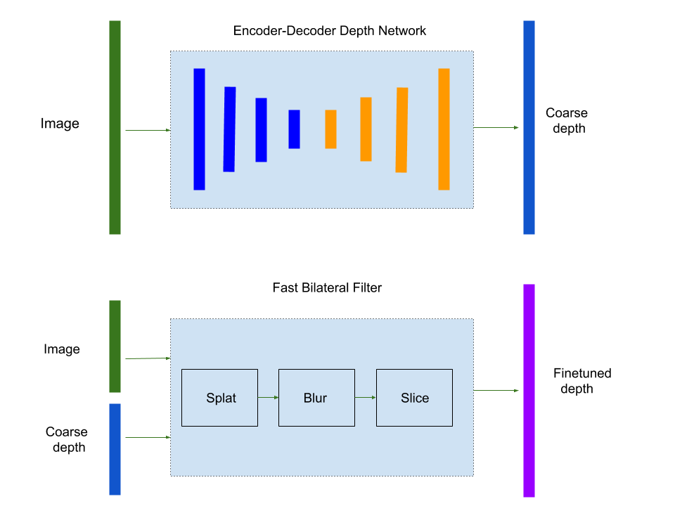
Nod.AI uses an encoder-decoder network to do a coarse depth estimation given an image. Then a bilateral filter is applied to finetune the depth map.

Nod.AI’s fast bilateral filter takes the input RGB image as a “reference” image and has the predicted depth map as “target value” t and some per-pixel confidence of the depth map c. The goal is to finetune the input depth map by resembling the input depth map where the confidence is large while being smooth and tightly aligned to edges in the reference image.

Nod.AI adopts “splat/blur/slice” procedures to speed up the bilateral filtering. Pixel values are “splatted” onto a small set of vertices in a grid or lattice (a soft histogramming operation), then those vertex values are blurred, and then the filtered pixel values are produced via a “slice” (an interpolation) of the blurred vertex values.

Nod.AI does the self-supervised depth training with monocular image sequences. During the training, we train a depth network which supports multiple popular backbones like Mobilenet and ResNet, and trains a separate pose network at the same time. The pose network predicts translation and rotation between a pair of image frames.

To formulate the training loss, we try to minimize the approximate photometric reprojection error between the predicted synthetic image and the target image. As the figure is shown below, we express the relative 6-DOF pose for the source image It’, with respect to the target image It ‘s pose as Tt->t’. After we get the depth map Dt of the target image, we can minimize the photometric reprojection error Lphoto:

 Lphoto = pe(It, It’->t)

It’->t = It’<proj(Dt, Tt->t’, K)>

Where pe is the photometric reprojection error; proj operator projects depths Dt onto 2D coordinates in It’ with pose Tt->t’  and intrinsics K

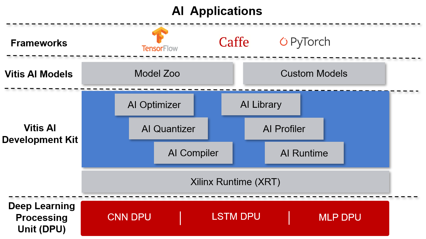
The Vitis AI development environment accelerates AI inference on Xilinx hardware platforms, including both edge devices and Alveo accelerator cards. It consists of optimized IP cores, tools, libraries, models, and example designs. It is designed with high efficiency and ease of use in mind, unleashing the full potential of AI acceleration on Xilinx FPGA and on the adaptive compute acceleration platform (ACAP). It makes it easier for users without FPGA knowledge to develop deep-learning inference applications, by abstracting away the intricacies of the underlying FPGA and ACAP.

The Xilinx Deep Learning Processor Unit (DPU) is a programmable engine dedicated to convolutional neural networks. The unit contains a register configure module, data controller module, and convolution computing module. There is a specialized instruction set for DPU, which enables DPU to work efficiently for many convolutional neural networks. The DPU IP can be integrated as a block in the programmable logic (PL) of the selected Zynq-7000 SoC and Zynq UltraScale + MPSoC devices with direct connections to the processing system (PS).

Nod.AI deploys the depth estimation solution on Xilinx edge devices including ZCU102 and ZCU104. The depth estimation solution can also be deployed on cloud devices like Alveo U50.

We mostly follow the Xilinx Vitis AI user guide (/content/xilinx/en/support/documentation/sw_manuals/vitis_ai/1_0/ug1414-vitis-ai.pdf) and Vitis AI library (https://github.com/Xilinx/Vitis-AI) during the model deployment. Like how the example code does with ResNet-50, we deploy the depth estimation model with the following four steps:

Quantize the neural network model

We modify the vai_q_tensorflow script to quantize the TensorFlow frozen depth model. Although the user guide suggests that calibrating the model with training images would achieve the best results, we found that in the case where we deployed the depth estimation model, calibrating neural network with random data achieve the best performance, and calibrating with a subset of training data tends to make the post-quantization model overfit.

Compile the neural network model

Vitis AI provides vai_c_tensorflow.py to compile the post-quantization model. You may meet the issue that your quantization was successful but the compiler fails and report an error message like this:

**************************************************

* VITIS_AI Compilation - Xilinx Inc.

**************************************************

/opt/vitis_ai/compiler/arch/dpuv2/ZCU102/ZCU102.json

[libprotobuf FATAL /home/dnnc/3rd-party/google/protobuf/repeated_field.h:1182] CHECK failed: (index) < (current_size_):

terminate called after throwing an instance of 'google::protobuf::FatalException'

  what():  CHECK failed: (index) < (current_size_):

Most likely it is because there were some operators like casting data type to float and multiplication in the model. After removing these operators, the model can be compiled successfully.

Program with Vitis AI programming interface

Vitis AI provides Unified C++ and Python APIs for Edge and Cloud to deploy models on FPGAs. After compilation, the elf file was generated and we can link it in the program and call DpuRunner to do the model inference.

Vitis AI runtime APIs are pretty straightforward. Most computer vision-related tasks need to use the OpenCV library. Fortunately, Xilinx has a built-in OpenCV library that is ready and sufficient to use.

Currently, DNNDK and Vitis AI reside together in the library. We met a mismatch performance between the post-quantization model and the compiled model problem when programming with DNNDK during the deployment. We found that it is because the input tensor has to be scaled with the value from dpuGetInputTensorScale() API and the output tensor has to be scaled with the value from dpuGetOutputTensorScale() API.

The depth estimation model has several operators that Vitis AI hasn’t supported yet so we have to implement it by ourselves. For example, we implemented the sigmoid layer that is applied to the last layer of the model

 Run and evaluate the deployed DPU application

It’s not always easy to deploy a model successfully even you follow the above steps. Sometimes we need to modify the model structure to fix some performance downgrade issues.

During our first deployment, we met a significant performance downgrade of the post-quantization model. We found that we need to replace the BiasAdd of Conv2D with the Batchnorm operation to make it more quantize-friendly. The example code is shown below:

In training:

output = tf.nn.relu(tf.layers.batch_normalization(conv2d(input, weights), training=True))

In inference and evaluation:

output = tf.nn.relu(tf.layers.batch_normalization(conv2d(input, weights), training=False))

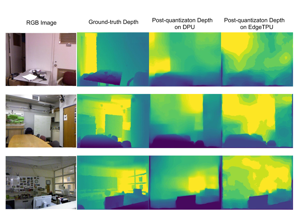
Below shows a comparison between the depth performance of the original TensorFlow float32 model, post-quantization model on DPU, and post-quantization model on EdgeTPU. Compared with EdgeTPU, DPU shows a cleaner depth map and better availability to preserve depth edges and depth details.

Accuracy

Speed

* GPU: Titan Xp

** CPU: Intel(R) Core(TM) i7-9750H CPU @ 2.60GHz

*** ZCU102 with 3x DPU B4096@300MHz. For the details about DPU, please refer to DPU Product Guide.

As we can see, we achieved the real-time inference speed with DPU running a compact embedded platform, which runs much faster than desktop CPU and EdgeTPU.

Comparing with Titan Xp which is a powerful desktop GPU, DPU shows 3.5-5.9x performance per watt advantage.

Performance:

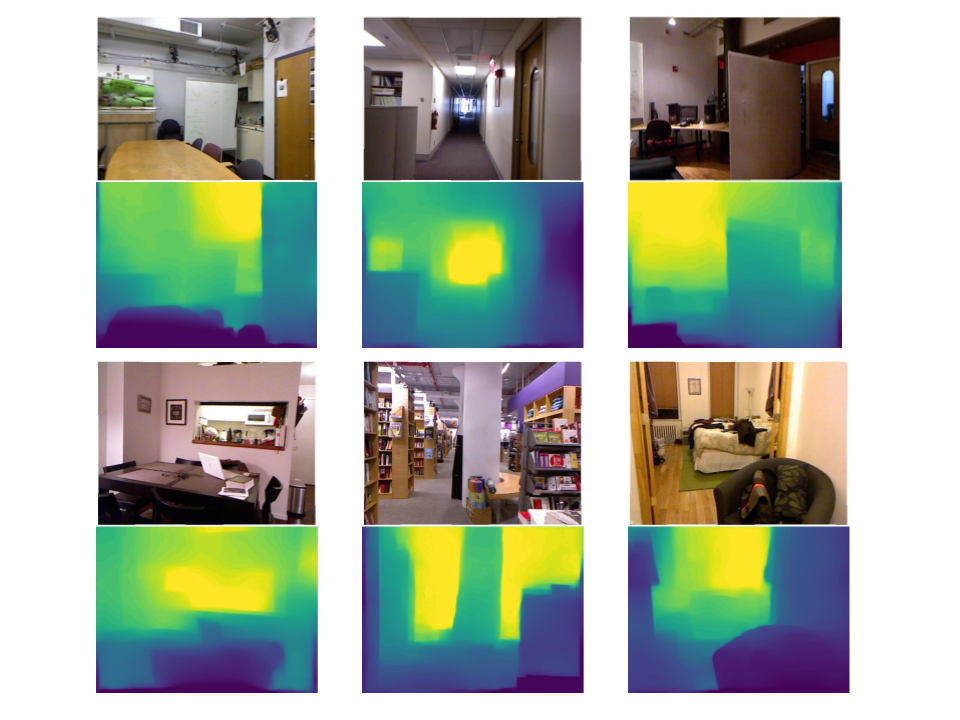
Below shows how Nod.AI depth estimation performs on Xilinx’s ZCU104 boards. The depth is painted to show the distance: the closer the darker, the farther the brighter.

-        Keep pushing the accuracy and scalability

-        Support higher resolution

-        Improve the post-quantization model accuracy

-        Utilize the model neural network search and pruning to further speed up the model inference

[1]:Huan Fu, Mingming Gong, Chaohui Wang, Kayhan Batmanghelich, and Dacheng Tao. Deep ordinal regression network for monocular depth estimation. In CVPR, pages 2002–2011, 2018.

[2]:Linda Wang, Mahmoud Famouri, and Alexander Wong. DepthNet Nano: A Highly Compact Self-Normalizing Neural Network for Monocular Depth Estimation. In CVPR, 2020.

[3]:Junsheng Zhou, Yuwang Wang, Kaihuai Qin, and Wenjun Zeng. Moving indoor: Unsupervised video depth learning in challenging environments. In ICCV, pages 8618–8627, 2019.

[4]:Wang Zhao Shaohui Liu Yezhi Shu Yong-Jin Liu. Towards Better Generalization: Joint Depth-Pose Learning without PoseNet. In CVPR, 2020.